Quantum mechanics - Density functional theory

Theory > Quantum_mechanics Theory-Quantum_mechanics

Created At : 2024-04-01 15:16

Count:190 Views 👀 :

04/30 2024
04/01/2024

Birds of a feather flock together.

物以类聚, 鸟以群分。

Updated time: 04/01 2024.

04/30 2024
Read the chapter 2 and 3.

Tomorrow I’ll read chapter 4. (It’s crucial for me)

In the festival, I’ll read the further reading list ASAP and quickly, just sketch reading.

Next week, I’ll do the practice all.

04/01/2024
0. Preface

Reading list

Focus solely on one DFT method suitable for solids and spatially extended materials, namely plane-wave DFT

A series of exercises at the end of chapter

1. What is Density Functional Theory
1.1 The Schrodinger equation

Ground state

Born-Oppenheimer approximation (approximation 1)

Adiabatic potential energy surface

$H\psi=E\psi$
$H$ - the Hamiltonian operator, not only one

$\psi$ - a set of solutions/ eigenstates of Hamiltonian

$E$ - real number. Each of these solutions, ${\psi _n}$, has an associated eigenvalue, ${E _n}$

1.2 The particle in a box or a harmonic oscillator
$\left[-\frac{\hbar^{2}}{2 m} \sum_{i=1}^{N} \nabla_{i}^{2}+\sum_{i=1}^{N} V\left(\mathbf{r}_{i}\right)+\sum_{i=1}^{N} \sum_{j<i} U\left(\mathbf{r}_{i}, \mathbf{r}_{j}\right)\right] \psi=E \psi$

left

the kinetic energy of each electron

the interaction energy between each electron and the collection of atomic nuclei

the interaction energy between different electrons

For this $H$, $\psi$ is electronic wave function, $\psi=\psi(\mathbf{r}_{1},\ldots,\mathbf{r}_{N})$. $E$ is ground state energy of the electrons (time-independent).

Hartree product (approximation 2)

Although the electron wave function is a function of each of the coordinates of all N electrons, it is possible to approximate $\psi$ as a product of individual electron wave functions.

$\psi=\psi_1(\mathbf{r})\psi_2(\mathbf{r}),\ldots,\psi_N(\mathbf{r})$

There are good motivations for approximating the full wave function into a product of individual one electron wave functions in this fashion.

Notice that $N$, the number of electrons, is considerably larger than $M$, the number of nuclei, simply because each atom has one nucleus and lots of electrons.

The dimension of full wave function for CO~2~ ($3·22=66$) , 100 Pt atoms (more than 23,000)

Why it’s many-body problem

The term in the Hamiltonian defining electron–electron interactions is the most critical one from the point of view of solving the equation.

The form of this contribution means that the individual electron wave function we defined above, $\psi_{i}(\mathbf{r})$, cannot be found without simultaneously considering the individual electron wave functions associated with all the other electrons.

Although solving the Schrodinger equation can be viewed as the fundamental problem of quantum mechanics, it is worth realizing that the wave function for any particular set of coordinates cannot be directly observed. The quantity that can (in principle) be measured is the probability that the N electrons are at a particular set of coordinates, $\mathbf{r}_{1},…,\mathbf{r}_{N} $. This probability is equal to $\psi^*(\mathbf{r}_1,\ldots,\mathbf{r}_N)\psi(\mathbf{r}_1,\ldots,\mathbf{r}_N)$, where the asterisk indicates a complex conjugate.

1.3 Do not care the order - electronic exchange
$n(\mathbf{r})=2\sum_i\psi_i^*(\mathbf{r})\psi_i(\mathbf{r})$

The factor of 2 appears because electrons have spin and the Pauli exclusion principle states that each individual electron wave function can be occupied by two separate electrons provided they have different spins.

the electron density, $n(r)$, which is a function of only three coordinates, contains a great amount of the information that is actually physically observable from the full wave function solution to the Schrodinger equation, which is a function of 3N coordinates.

1.4 From wave functions to electron density

Two fundamental mathematical theorems proved by Kohn and Hohenberg

The ground-state energy from Schrodinger’s equation is a unique functional of the electron density.

There exists a one-to-one mapping between the ground-state wave function and the ground-state electron density.

So we can restate Hohenberg and Kohn’s result by saying that the ground-state energy E can be expressed as $E[n(r)]$, where $n(r)$ is the electron density. This is why this field is known as density functional theory.

Another way to restate Hohenberg and Kohn’s result is that the ground-state electron density uniquely determines all properties, including the energy and wave function, of the ground state. Why is this result important? It means that we can think about solving the Schrodinger equation by finding a function of three spatial variables, the electron density, rather than a function of 3N variables, the wave function.

Unfortunately, although the first Hohenberg–Kohn theorem rigorously proves that a functional of the electron density exists that can be used to solve the Schrodinger equation, the theorem says nothing about what the functional actually is.

The electron density that minimizes the energy of the overall functional is the true electron density corresponding to the full solution of the Schrodinger equation.

A useful way to write down the functional described by the Hohenberg–Kohn theorem is in terms of the single-electron wave functions, $\psi_i(r)$.
$E[\{\psi_i\}]=E_\text{known}[\{\psi_i\}]+E_\text{XC}[\{\psi_i\}]$ $\begin{aligned}E_\text{known}[\{\psi_i\}]&=-\frac{\hbar^2}{m}\sum_i\int\psi_i^*\nabla^2\psi_id^3r+\int V(\textbf{r})n(\textbf{r})d^3r\\&+\frac{e^2}{2}\int\int\frac{n(\textbf{r})n(\textbf{r}')}{|\textbf{r}-\textbf{r}'|}d^3rd^3r'+E_\text{ion}.\end{aligned}$

Right: the electron kinetic energies, the Coulomb interactions between the electrons and the nuclei, the Coulomb interactions between pairs of electrons, and the Coulomb interactions between pairs of nuclei.

The other term in the complete energy functional, $E_{XC}[\{\psi_i\}]$, is the exchange–correlation functional, and it is defined to include all the quantum mechanical effects that are not included in the “known” terms.

What is involved in finding minimum energy solutions of the total energy functional?

The derivation of a set of equations by Kohn and Sham

This difficulty was solved by Kohn and Sham, who showed that the task of finding the right electron density can be expressed in a way that involves solving a set of equations in which each equation only involves a single electron.

The Kohn-Sham equations
$\left[-\frac{\hbar^2}{2m}\nabla^2+V(\mathbf{r})+V_H(\mathbf{r})+V_{\mathrm{XC}}(\mathbf{r})\right]\psi_i(\mathbf{r})=\varepsilon_i\psi_i(\mathbf{r}).$

Missing the summations that appear inside the full Schrodinger equation. This is because the solution of the Kohn–Sham equations are single-electron wave functions that depend on only three spatial variables, $\psi_i(r)$.

Hartree potential $V_H(\mathbf{r})=e^2\int\frac{n(\mathbf{r}’)}{|\mathbf{r}-\mathbf{r}’|}d^3r’$. This potential describes the Coulomb repulsion between the electron being considered in one of the Kohn–Sham equations and the total electron density defined by all electrons in the problem. The Hartree potential includes a so-called self-interaction (unphysical) contribution because the electron we are describing in the Kohn–Sham equation is also part of the total electron density, so part of $V_H$ involves a Coulomb interaction between the electron and itself.

The correction, $V_{XC}$, which defines exchange and correlation contributions to the single electron equations. $V_{\mathrm{XC}}(\mathbf{r})=\frac{\delta E_{\mathrm{XC}}(\mathbf{r})}{\delta n(\mathbf{r})}$

If you have a vague sense that there is something circular about our discussion of the Kohn–Sham equations you are exactly right. To solve the Kohn–Sham equations, we need to define the Hartree potential, and to define the Hartree potential we need to know the electron density. But to find the electron density, we must know the single-electron wave functions, and to know these wave functions we must solve the Kohn–Sham equations. To break this circle, the problem is usually treated in an iterative way as outlined in the following algorithm:

Define an initial, trial electron density, $n(r)$.

Solve the Kohn–Sham equations defined using the trial electron density to find the single-particle wave functions, $\psi_i(r)$.

Calculate the electron density defined by the Kohn–Sham single-particle wave functions from step 2, $n_{\mathrm{KS}}(\mathbf{r})=2\sum_{i}\psi_{i}^{*}(\mathbf{r})\psi_{i}(\mathbf{r})$

Compare the calculated electron density, $n_{KS}(r)$, with the electron density used in solving the Kohn–Sham equations, $n(r)$. If the two densities are the same, then this is the ground-state electron density, and it can be used to compute the total energy. If the two densities are different, then the trial electron density must be updated in some way. Once this is done, the process begins again from step 2.

We have skipped over a whole series of important details in this process

How close do the two electron densities have to be before we consider them to be the same?

What is a good way to update the trial electron density?

How should we define the initial density?

1.5 Exchange-correlation functional, $E_{XC}[\{\psi_i\}]$

Fortunately, there is one case where this functional can be derived exactly: the uniform electron gas (the electron density is constant at all points in space, $n(r) = constant$) (approximation 3)

This situation may appear to be of limited value in any real material since it is variations in electron density that define chemical bonds and generally make materials interesting.

we set the exchange–correlation potential at each position to be the known exchange–correlation potential from the uniform electron gas at the electron density observed at that position.
$V_{\mathrm{XC}}(\mathbf{r})=V_{\mathrm{XC}}^{\text{electron gas}}[n(\mathbf{r})]$

This approximation uses only the local density to define the approximate exchange–correlation functional, so it is called the local density approximation (LDA).

The best known class of functional after the LDA uses information about the local electron density and the local gradient in the electron density; this approach defines a generalized gradient approximation (GGA). It is tempting to think that because the GGA includes more physical information than the LDA it must be more accurate. Unfortunately, this is not always correct.

Two of the most widely used functionals in calculations involving solids are the Perdew–Wang functional (PW91) and the Perdew–Burke–Ernzerhof functional (PBE).

Because different functionals will give somewhat different results for any particular configuration of atoms, it is necessary to specify what functional was used in any particular calculation rather than simple referring to “a DFT calculation.”

Our description of GGA functionals as including information from the electron density and the gradient of this density suggests that more sophisticated functionals can be constructed that use other pieces of physical information. In fact, a hierarchy of functionals can be constructed that gradually include more and more detailed physical information.

1.6 The Quantum Chemistry Tourist

Localized and Spatially Extended Functions

Spatially localized functions

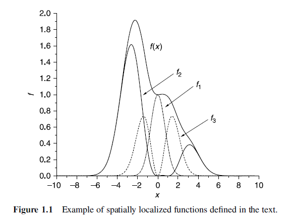
Spatially localized functions are an extremely useful framework for thinking about the quantum chemistry of isolated molecules because the wave functions of isolated molecules really do decay to zero far away from the molecule.

Spatially Extended functions

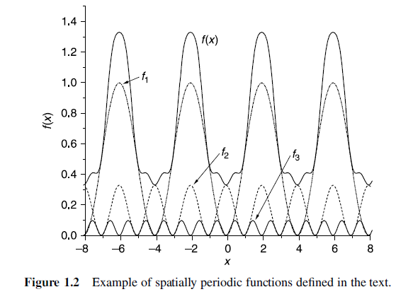
We could still use spatially localized functions to describe each atom and add up these functions to describe the overall material, but this is certainly not the only way forward.
A useful alternative is to use periodic functions to describe the wave functions or electron densities.

This type of function is useful for describing bulk materials since at least for defect-free materials the electron density and wave function really are spatially periodic functions.

Because spatially localized functions are the natural choice for isolated molecules, the quantum chemistry methods developed within the chemistry community are dominated by methods based on these functions. Conversely, because physicists have historically been more interested in bulk materials than in individual molecules, numerical methods for solving the Schrodinger equation developed in the physics community are dominated by spatially periodic functions.

Wave-Function-Based Methods

The quantity that is being calculated: electron density/the full electron wave function

These wave-function-based methods hold a crucial advantage over DFT calculations in that there is a well-defined hierarchy of methods that, given infinite computer time, can converge to the exact solution of the Schrodinger equation. 😂

These wave functions must satisfy several mathematical properties exhibited by real electrons. For example, the Pauli exclusion principle prohibits two electrons with the same spin from existing at the same physical location simultaneously.

Hartree-Fock Method

We would like to approximate the wave function of N electrons. Let us assume for the moment that the electrons have no effect on each other (we simply neglect electron–electron interactions).

The Hamiltonian $H=\sum_{i=1}^Nh_i$

The Schrodinger equation $h\chi=E\chi$

The eigenfunctions - spin orbitals, $\chi_j(x_i)(j=1, 2, …)$, energy $E_j$

$x_i$ is a vector of coordinates that defines the position of electron $i$ and its spin state (up and down)

$j=1$ the lowest energy, $j=2$ next highest energy
$\psi(\mathbf{x}_1,\ldots,\mathbf{x}_N)=\chi_{j_1}(\mathbf{x}_1)\chi_{j_2}(\mathbf{x}_2)\cdots\chi_{j_N}(\mathbf{x}_N)$ $E=E_{j1}+...+E_{jN}$

The Hartree product does not satisfy all the important criteria for wave functions. Because electrons are fermions, the wave function must change sign if two electrons change places with each other. This is known as the antisymmetry principle. Exchanging two electrons does not change the sign of the Hartree product, which is a serious drawback.

The Slater determinant - a better approximation to the wave function to spin orbitals

In a Slater determinant, the N-electron wave function is formed by combining one-electron wave functions in a way that satisfies the antisymmetry principle. This is done by expressing the overall wave function as the determinant of a matrix of single-electron wave functions.

$\psi(\mathbf{x}_1,\mathbf{x}_2)=\dfrac{1}{\sqrt{2}}\det\begin{bmatrix}\chi_j(\mathbf{x}_1)&\chi_j(\mathbf{x}_2)\\\chi_k(\mathbf{x}_1)&\chi_k(\mathbf{x}_1)\end{bmatrix} =\frac{1}{\sqrt{2}}\Big[\chi_j(\mathbf{x}_1)\chi_k(\mathbf{x}_1)-\chi_j(\mathbf{x}_2)\chi_k(\mathbf{x}_1)\Big].$

$\dfrac{1}{\sqrt{2}}$ - a normalization factor

The Slater determinant satisfies the conditions of the Pauli exclusion principle

This expression builds in a physical description of electron exchange implicitly;

It changes sign if two electrons are exchanged.

This expression has other advantages. For example, it does not distinguish between electrons and it disappears if two electrons have the same coordinates or if two of the one-electron wave functions are the same.

The Slater determinant may be generalized to a system of N electrons easily; it is the determinant of an $N\times N$ matrix of single-electron spin orbitals.

The Hartree-Fock method (the simplest approach, considering the electron–electron interactions)

we fix the positions of the atomic nuclei and aim to determine the wave function of N-interacting electrons.

For each electron

$\left[-\frac{\hbar^2}{2m}\nabla^2+V(\mathbf{r})+V_H(\mathbf{r})\right]\chi_j(\mathbf{x})=E_j\chi_j(\mathbf{x})\\ V_H(\mathbf{r})=e^2\int\frac{n(\mathbf{r}')}{|\mathbf{r}-\mathbf{r}'|}d^3r'$

this means that a single electron “feels” the effect of other electrons only as an average, rather than feeling the instantaneous repulsive forces generated as electrons become close in space. the average field, the classical electrostatic potential.

If you compare with the Kohn–Sham equations, you will notice that the only difference between the two sets of equations is the additional exchange–correlation potential that appears in the Kohn–Sham equations.

The HF approach assumes that the complete wave function can be approximated using a single Slater determinant. This means that the N lowest energy spin orbitals of the single-electron equation are found, $\chi_j(x)$ for $j=1,…,N$, and the total wave function is formed from the Slater determinant of these spin orbitals.

define the spin orbitals using a finite set of functions

$\chi_j(\mathbf{x})=\sum_{i=1}^K\alpha_{j,i}\phi_i(\mathbf{x})$

When using this expression, we only need to find the expansion coefficients, $\alpha_{j,i}$, for $i=1,…,K$ and $j=1,…,N$ to fully define all the spin orbitals that are used in the HF method. The set of functions $\phi_1(x),\phi_2(x),…,\phi_K(x)$ is called the basis set for the calculation.

We now have all the pieces in place to perform an HF calculation—a basis set in which the individual spin orbitals are expanded, the equations that the spin orbitals must satisfy, and a prescription for forming the final wave function once the spin orbitals are known. But there is one crucial complication left to deal with; one that also appeared when we discussed the Kohn–Sham equations. To find the spin orbitals we must solve the single electron equations. To define the Hartree potential in the single-electron equations, we must know the electron density. But to know the electron density, we must define the electron wave function, which is found using the individual spin orbitals! To break this circle, an HF calculation is an iterative procedure that can be outlined as follows:

Make an initial estimate of the spin orbitals $\chi_j(\mathbf{x})=\sum_{i=1}^K\alpha_{j,i}\phi_i(\mathbf{x})$ by specifying the expansion coefficients, $\alpha_{j,i}$

From the current estimate of the spin orbitals, define the electron density, $n(\mathbf{r}^{\prime})$

Using the electron density from step 2, solve the single-electron equations for the spin orbitals.

If the spin orbitals found in step 3 are consistent with orbitals used in step 2, then these are the solutions to the HF problem we set out to calculate. If not, then a new estimate for the spin orbitals must be made and we then return to step 2.

Questions

How do we decide if two sets of spin orbitals are similar enough to be called consistent?

How can we update the spin orbitals in step 4. so that the overall calculation will actually converge to a solution?

How large should a basis set be? How can we form a useful initial estimate of the spin orbitals?

How do we efficiently find the expansion coefficients that define the solutions to the single-electron equations?

Beyond Hartree–Fock (add electron correlations) (the level of theory and the basis set)

The Hartree–Fock method provides an exact description of electron exchange (femions)

If HF calculations were possible using an infinitely large basis set, the energy of N electrons that
would be calculated is known as the Hartree–Fock limit

HF, This energy is not the same as the energy for the true electron wave function because the
HF method does not correctly describe how electrons influence other electrons. More succinctly, the HF method does not deal with electron correlations (crucial for molecular system). $V_{XC}$

single-determinant methods

post-Hartree-Fock methods

configuration interaction (CI)

coupled cluster (CC)

CCSD - coupled-cluster calculations involving excitations of single electrons (S),
and pairs of electrons (double—D)

CCSDT - further include excitations of three electrons (triples—T)

Moller–Plesset perturbation theory (MP)

adding a small perturbation (the correlation potential) to a zero order Hamiltonian (the HF Hamiltonian, usually)

a number is used to indicate the order of the perturbation theory, so MP₂ is the second-order theory and so on.

the quadratic configuration interaction (QCI) approach

The reference wave function

Multiconfigurational self-consistent field (MCSCF)

Multireference single and double configuration interaction (MRDCI)

N-electron valence state perturbation theory (NEVPT) methods.

For a basis set with N functions, the computational expense

HF: ~N⁴

CC: ~N⁷

Moreover, we will only consider methods based on spatially periodic functions—the so-called plane-wave methods. Plane-wave methods are the method of choice in almost all situations where the physical material of interest is an extended crystalline material rather than an isolated molecule.

Perhaps the main difference between DFT calculations using periodic and spatially localized functions lies in the exchange–correlation functionals that are routinely used.

The most commonly used functionals in DFT calculations based on spatially localized basis functions are “hybrid” functionals that mix the exact results for the exchange part of the functional with approximations for the correlation part.

Unfortunately, the form of the exact exchange results mean that they can be efficiently implemented for applications based on spatially localized functions but not for applications using periodic functions!

Because of this fact, the functionals that are commonly used in plane-wave DFT calculations do not include contributions from the exact exchange results.

1.7 What can DFT not do?

The first situation where DFT calculations have limited accuracy is in the calculation of electronic excited states

Underestimation of calculated band gaps in semiconducting and insulating materials

The DFT calculations give inaccurate results is associated with the weak van der Waals (VDW) attractions that exist between atoms and molecules.

There is one more fundamental limitation of DFT that is crucial to appreciate, and it stems from the computational expense associated with solving the mathematical problem posed by DFT.

1.8 Further reading

无机化学

结构化学基础

固体物理导论 (Introduction to solid states)

Quantum Chemistry

Electronic Structure: Basic Theory and Practical Methods

Please indicate the source when reprinting. Please verify the citation sources in the article and point out any errors or unclear expressions.